How to Extract Only Numbers from Text Fields in Google Sheets Using REGEXEXTRACT and ARRAYFORMULA?
Sometimes your data comes messy — like “42 Nos”, “205 Nos”, “1 Nos”, and you just want the pure numbers.
Manually cleaning each line? Not happening.
Luckily, Google Sheets gives us a super clean way to fix it in one shot using REGEXEXTRACT and ARRAYFORMULA.
Here’s exactly how.
The Problem
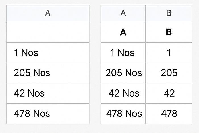
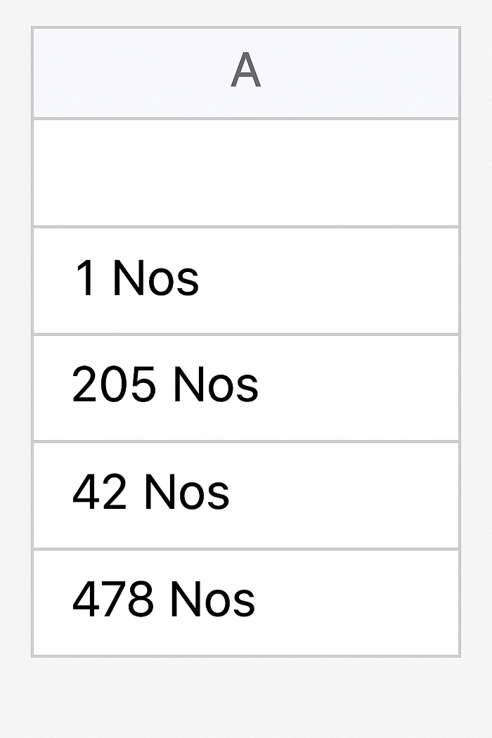
You have data like this:
You want it to look like this:
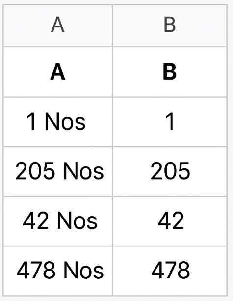
Column B is clean, number-only.
The Formula
Here’s the exact formula you’ll use:
=ARRAYFORMULA(IF(A:A<>"", VALUE(REGEXEXTRACT(A:A, "\d+")), ""))
✅ Put it in B1.
✅ Done.
What’s Actually Happening
REGEXEXTRACT(A:A, "\d+"): Pulls out the first set of digits it finds. (Here, the numbers.)VALUE(...): Converts the extracted text to a real number so it behaves like a number (not just looks like one).ARRAYFORMULA(...): Applies the logic to the entire column at once, no dragging down needed.
Why Not Just Use SPLIT or LEFT?
You could try messy ways with SPLIT, LEFT, etc., but:
- If the text structure changes later (maybe spaces, different wording), your formulas break.
- Regex is bulletproof. If there are digits, it catches them. Always.
Clean, scalable, future-proof.
Quick Example
Imagine you now paste 10,000 rows of “Item Nos” into your Sheet.
✅ With this setup, the numbers show automatically.
✅ No rework.
✅ No formulas to drag.
✅ No worrying about extra spaces or typos.
In short:
If you need to rip numbers out of messy text columns in Google Sheets —
ARRAYFORMULA + REGEXEXTRACT is the fastest, cleanest way.
Save this formula.
Use it everywhere